Soft actor-critic with auto H.O.
TL;DR:
- Based on the idea of
Soft Actor-Critic, this paper includes a constrained formulation that automatically tunes the temperature hyperparameter. - Revised version of soft actor-critic also shows state-of-the-art performance in sample-efficiency and asymptotic performance while retaining the benefits of entropy maximization and stability without any environment specific hyperparameter tuning.
- Soft actor-critic is robust and sample efficient enough for robotic tasks learned directly in the real world, such as locomotion and dexterous manipulation.
This review only deals with automating entropy adjustment part of the paper. If you want to know basic idea of soft actor-critic, please see Soft Actor-Critic post.
Automating Entropy Adjustment for Maximum Entropy RL
Previous soft actor-critic learns maximum entropy policies of a given temperature. Instead of requiring the user to set the temperature manually, we can automate this process by a constrained optimization problem where the average entropy of the policy is constrained, while the entropy at different states can vary. The dual to this constrained optimization leads to the soft actor-critic updates, along with an additional update for the dual variable, which plays the role of the temperature. At first, this paper derive the update for finite horizon case, and then derive an approximation for stationary policies by dropping the time dependencies from the policy, soft Q-function, and the temperature.
Constrained optimization problem in finite horizon
The goal is to find a stochastic policy with maximal expected return that satisfies a minimum expected entropy constraint. The constrained optimization problem is
\[\begin{equation}\label{eqn:const-prob} \underset{\pi_{0:T}}{\mathrm{max}} \ \mathbb E_{\rho_\pi} \left[ \sum_{t=0}^T r(s_t,a_t) \right] \quad \mathrm{s.t.} \ \mathbb E_{(s_t,a_t) \sim \rho_\pi} \left[ -\mathrm{log}(\pi_t(a_t \mid s_t)) \right] \geq \mathcal H \quad \forall t \end{equation}\]where \(\mathcal H\) is a desired minimum expected entropy (equals to minus of entropy target in the Table 1 from Appendix D). Since the policy at time \(t\) can only affect the future objective value, we rewrite the objective as an iterative maximization
\[\begin{equation} \underset{\pi_0}{\mathrm{max}} \left( \mathbb E \left[ r(s_0,a_0) \right] + \underset{\pi_1}{\mathrm{max}} \left( \mathbb E\left[...\right] + \underset{\pi_T}{\mathrm{max}}\ \mathbb E \left[r(s_T,a_T)\right] \right) \right), \end{equation}\]subject to the constraint on entropy. Starting from the last time step, we change the constrained maximization to the dual problem. Subject to \(\mathbb E_{(s_t,a_t) \sim \rho_\pi} \left[ -\mathrm{log} (\pi_T(a_T \mid s_T)) \right] \geq \mathcal H\),
\[\begin{equation} \underset{\pi_T}{\mathrm{max}}\ \mathbb E_{(s_T,a_T) \sim \rho_\pi} \left[r(s_T,a_T)\right] = \underset{\alpha_T \geq 0}{\mathrm{min}}\ \underset{\pi_T}{\mathrm{max}}\ \mathbb E \left[r(s_T,a_T) - \alpha_T\ \mathrm{log}\ \pi(a_T \mid s_T)\right] - \alpha_T \mathcal H, \end{equation}\]where \(\alpha_T\) is the dual variable. Since the objective is linear and the entropy constraint is convex function in \(\pi_T\) , strong duality holds. This dual objective is closely related to the maximum entropy objective with respect to the policy, and the optimal policy is the maximum entropy policy coresponding to the temperature \(\alpha_T : \pi_T^* (a_T \mid s_T;\alpha_T)\) . We can solve for the optimal dual variable \(\alpha_T^*\) as
\[\begin{equation} \underset{\alpha_T}{\mathrm{argmin}}\ \mathbb E_{(s_t,a_t) \sim \pi_t^* } \left[ -\alpha_T \mathrm{log}\ \pi_T^* (a_T \mid s_T;\alpha_T) - \alpha_T \mathcal H \right]. \end{equation}\]To simplify notation, we make use of the recursive definition of the soft Q-function
\[\begin{equation} Q_t^* (s_t,a_t; \pi_{t+1:T}^* , \alpha_{t+1:T}^* ) = \mathbb E \left[r(s_t,a_t)\right] + \mathbb E_{\rho_\pi} \left[Q_{t+1}^* (s_{t+1},a_{t+1}) - \alpha_{t+1}^* \ \mathrm{log}\ \pi_{t+1}^* (a_{t+1} \mid s_{t|1}) \right], \end{equation}\]with \(Q_T^* (s_T, a_T) = \mathbb E \left[ r(s_T, a_T) \right]\) . Now, subject to the entropy constraints and again using the dual problem, we have
\[\begin{align}\label{eqn:deploy-eqn} \begin{split} \underset{\pi_{T-1}}{\mathrm{max}} & \left( \mathbb E \left[ r(s_{T-1},a_{T-1}) \right] + \underset{\pi_T}{\mathrm{max}}\ \mathbb E \left[ r(s_T,a_T) \right] \right) \\ & = \underset{\pi_{T-1}}{\mathrm{max}}\ \left( \mathbb E \left[ r(s_{T-1},a_{T-1}) \right] + \underset{\alpha_T \geq 0}{\mathrm{min}}\ \underset{\pi_T}{\mathrm{max}}\ \mathbb E \left[ r(s_T,a_T) - \alpha_T\ \mathrm{log}\ \pi_T(a_T \mid s_T) \right] - \alpha_T \mathcal H \right) \\ & = \underset{\pi_{T-1}}{\mathrm{max}}\ \left( \mathbb E \left[ r(s_{T-1},a_{T-1}) \right] + Q_T^* (s_T,a_T) \right) \\ & = \underset{\pi_{T-1}}{\mathrm{max}}\ \left( \mathbb E \left[ r(s_{T-1},a_{T-1}) \right] + \mathbb E_{\rho_\pi} \left[ Q_T^* (s_T,a_T) - \alpha_T^* \ \mathrm{log}\ \pi_T^* (a_T \mid s_T) \right] - \alpha_T^* \mathcal H \right) \\ & = \underset{\pi_{T-1}}{\mathrm{max}}\ \left( Q_{T-1}^* (s_{T-1}, a_{T-1}) - \alpha_T^* \mathcal H \right) \\ & = \underset{\alpha_{T-1} \geq 0}{\mathrm{min}}\ \underset{\pi_{T-1}}{\mathrm{max}}\ \left( \mathbb E \left[ Q_{T-1}^* (s_{T-1},a_{T-1}) \right] - \mathbb E \left[ \alpha_{T-1}\ \mathrm{log}\ \pi_{T-1}(a_{T-1} \mid s_{T-1}) \right] - \alpha_{T-1} \mathcal H \right) - \alpha_T^* \mathcal H \end{split} \end{align}\]By applying the procedure (\ref{eqn:deploy-eqn}) to the constrained optimization problem recursively, we get
\[\begin{equation} \mathrm Eq. (\ref{eqn:const-prob}) = \mathbb E_{a_0 \sim \pi_0^* } \left[ Q_0^* (s_0,a_0)\right] - \sum_{t=0}^T \alpha_t^* \mathcal H. \end{equation}\]The summation term: \(-\sum_{t=0}^T \alpha_t^* \mathcal H\) is minus of the total entropy equals to the sum of entropy target weighted by \(\alpha_t^*\) for each time step. We can also include discount factor \(\gamma\) as usual. After solving for \(Q_t^*\) and \(\pi_t^*\) , we can solve the optimal dual variable \(\alpha_t^*\) as
\[\begin{equation}\label{eqn:alpha-opt} \alpha_t^* = \underset{\alpha_t}{\mathrm{argmin}}\ \mathbb E_{a_t \sim \pi_t^* } \left[ -\alpha_t\ \mathrm{log}\ \pi_t^* (a_t \mid s_t;\alpha_t) - \alpha_t \bar{\mathcal H} \right]. \end{equation}\]
Practical Algorithm
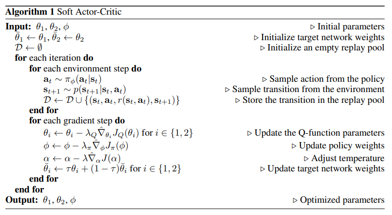
The complete algorithm is described in Algorithm 1.

In the previous version of soft actor-critic algorithm, they used an additional function approximator for the value function. But as it is found to be unnecessary, this algorithm only used two soft Q-function networks, their respective target networks and policy network parameters. In addition to the soft Q-function and the policy, learning \(\alpha\) by minimizing the dual objective in Equation (\ref{eqn:alpha-opt}). This can be done by approximating dual gradient descent. Dual gradient descent alternates between optimizing the Largrangian with respect to the primal variables to convergence(solving for \(Q_t^* , \pi_t^*\) ), and then taking a gradient step on the dual variables(solving for \(\alpha_t^*\) with \(Q_t^* , \pi_t^*\) ). As optimizing with respect to the primal variables fully is impractical, a truncated approach that performs incomplete optimization (even for a single gradient step) still works in practice. Thus, \(\alpha\) is updated with the following objective:
Experiment
Simulated Benchmarks

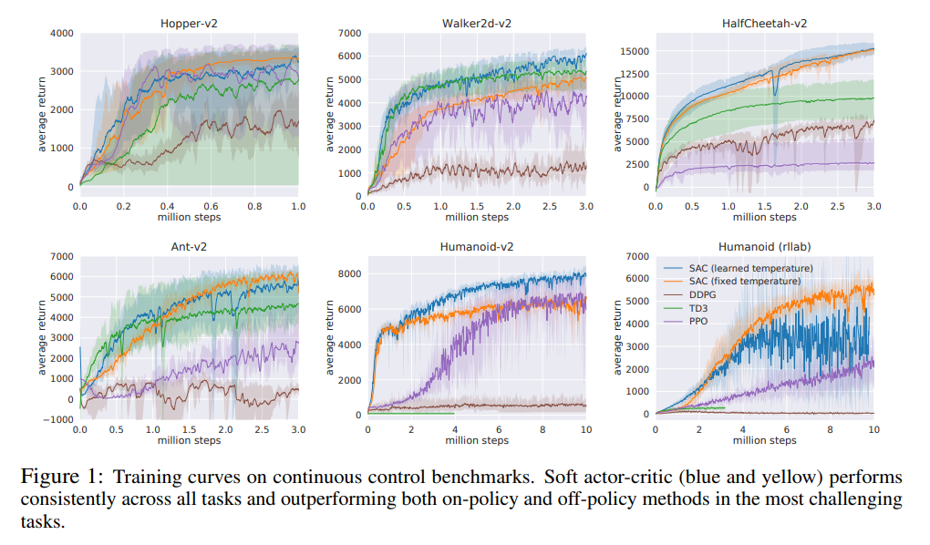
SAC performs comparably to the baseline methods on the easier tasks and outperforms them on the harder tasks with a large margin, both in terms of learning speed and the final performance. The results also show that the automatic temperature tuning scheme works well across all the environments, and thus, effectively eliminates the need for tuning the temperature.
Quadrupedal Locomotion in the Real World
Task specification
- Latencies and contacts in the system make the dynamics non-Markovian, which can significantly degrade learning performance. Therefore, they construct the state out of the current and past five observations and actions.
- Reward function rewards large forward velocity, penalizes large angular acceleration, large pitch angles and extending the front legs under the robot.
- Robot training pipeline consists of two components parallel jobs: training and data collection.
- Locomotion task (real-world reinforcement learning) is substantially challenging that an untrained policy can lose balance and fall, and too many falls will eventually damage the robot, making sample-efficient learning essentially.

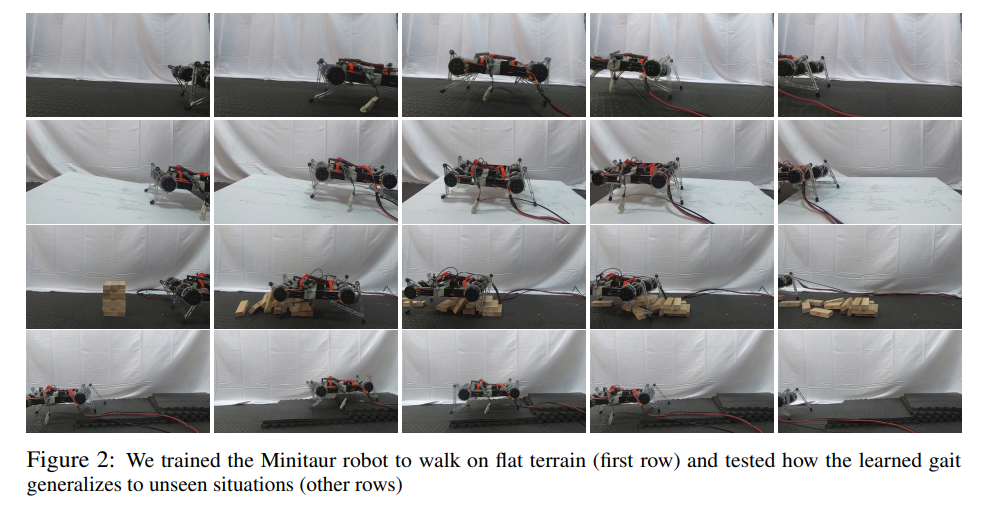
In the real world, the utility of a locomotion policy hinges critically on its ability to generalize to different terrains and obstacles. Because soft actor-critic learns robust policies, the results above show that the policy can readily generalize to these perturbation without any additional learning. This experiment is the first example of a deep reinforcement learning algorithm learning underactuated quadrupedal locomotion directly in the real world without any simulation or pretraining.
Dexterous Hand Manipulation
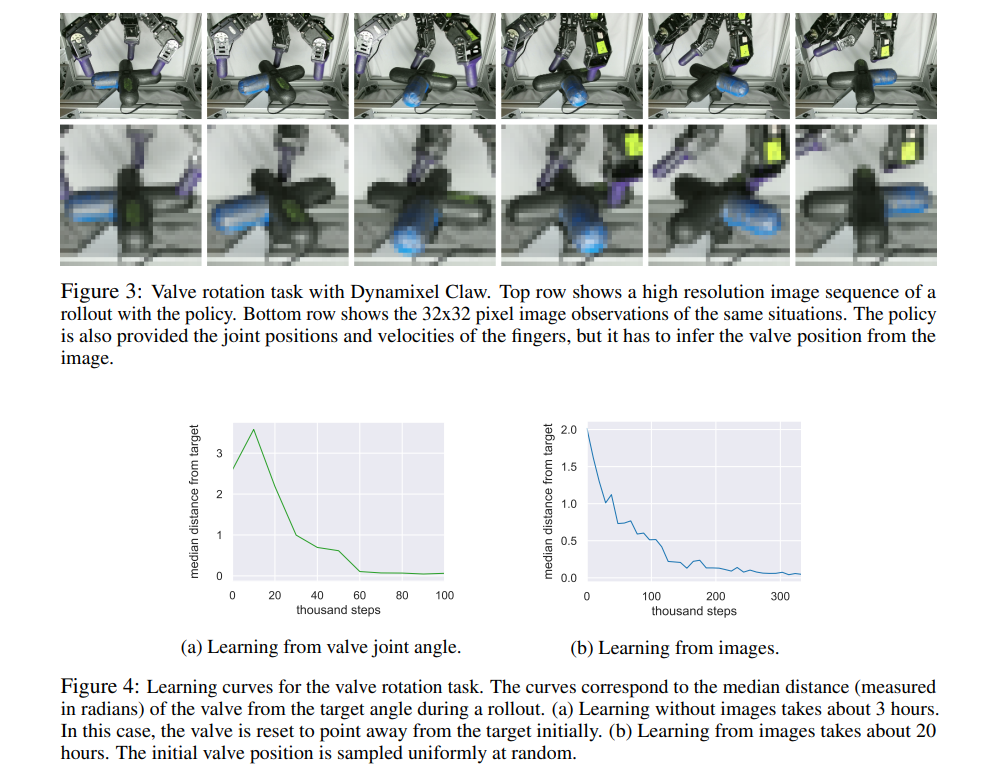
The manipulation task requires a 3-finger dexterous robotic hand(9-DOF) to rotate a “valve”-like object into the correct position, with the colored part of the valve facing directly to the right, from any random starting position. This task is exceptionally challenging due to both the perception challenges and the physical difficulty of rotating the valve with such a complex robotic hand.

This task represents one of the most complex robotic manipulation tasks learned directly end-to-end from raw images in the real world with deep reinforcement learning, without any simulation or pretraining. The results above also show that learning the same task by feeding the valve position directly to the neural networks takes 3 hours, which is substantially faster than PPO did (7.4 hours).
Discussion
- For the rllab humanoid task, the result of SAC with learned temperature highly oscillates compared with SAC with fixed temperature. Doesn’t it mean automatic temperature tuning is brittle to harder task?
- Also, SAC with learned temperature has worse asymptotic performance than SAC with fixed temperature. Considering this fact, can we still say that automatic temperature tuning scheme works well across all the enviroments?
- In the locomotion task, the paper describes how they define the reward function which aims to make the robot locomote well. I think it shows the importance of a good reward function. But, making a good reward function MANUALLY can be extremely harder for high-dimensional, abstract tasks. I think this problem pose the necessity of the research on Unsupervised RL or Inverse RL.
- If we see
the learned policy on the Dexterous Hand Manipulation task, robotic hand accomplishes the task well, without using the finger left in the video. There may be other videos that the robotic hand use its whole three fingers to rotate the valve. But considering that possibility, the movements of the robotic hand seem not good enough in the perspective of human.