Soft Actor-Critic
TL;DR:
- Soft Actor-Critic; an off-policy actor-critic deep RL algorithm based on the maximum entropy reinforcement learning framework
- SAC achieves SOTA performance on a range of continuous control benchmark tests, outperforming prior on-policy and off-policy method.
- SAC is very stable in contrast to other off-policy algorithms.
Introduction
Challenges on Model-free deep reinforcement learning (RL) algorithms
- Model-free deep RL methods are notoriously expensive in terms of their sample complexity.
- Model-free deep RL methods are often brittle with respect to their hyperparameters.
One cause for the poor sample efficiency is on-policy learning such as TRPO, PPO or A3C. In contrast to on-policy learning, off-policy algorithms aim to reuse past experience. Unfortunately, the combination of off-policy learning and high dimensional, nonlinear function approximation with neural networks presents a major challenge for stability and convergence(so-called deadly triad). This challenge is further exacerbated in continuous state and action spaces, where DDPG is in such settings. DDPG provides for sample-efficient learning but is notoriously challenging to use due to its extreme brittleness and hyperparameter sensitivity.
Maximum Entropy Framework
To solve these problems, the maximum entropy framework is used in this paper. The maximum entropy formulation provides a substantial improvement in exploration and robustness with a stochastic actor. Prior work has proposed off-policy algorithms based on soft Q-learning and its variants. However, the off-policy variants require complex approximate inference procedures in continuous action spaces(sampling network in Soft Q-Learning). In this paper, off-policy maximum entropy actor-critic algorithm (SAC) is devised. SAC avoids the complexity and potential instability associated with approximate inference in prior off-policy maximum entropy algorithms based on soft Q-learning.
Is Soft Q-learning is true actor-critic algorithm?
Although the soft Q-learning algorithm has a value function and actor network, it is not a true actor-critic algorithm: the Q-function is estimating the optimal Q-function, and the actor does not directly affect the Q-function except through the data distribution. Hence, soft Q-learning motivates the actor network as an approximate sampler rather than the actor in an actor-critic algorithm. While convergence of soft Q-learning depends on how well this sampler approximates the true posterior, SAC converges to the optimal policy from a given policy class, regardless of the policy parameterization.
Preliminaries
Maximum Entropy Reinforcement Learning
Maximum entropy objective with the expected entropy of the policy over \(\rho_\pi(s_t)\) :
\[\begin{equation} J(\pi) =\sum_{t=0}^\infty \mathbb E_{(s_t,a_t) \sim \rho_\pi} \left[\sum_{l=t}^\infty \gamma^{l-t} \mathbb E_{s_l \sim p,a_l \sim \pi} \left[r(s_t,a_t)+\alpha \mathcal H(\pi(\cdot|s_t)) \right]\right]. \end{equation}\]The temperature parameter \(\alpha\) determines the relative importance of the entropy term against the reward, and thus controls the stochasticity of the optimal policy. By adapting maximum entropy framework, the policy is incentivized to explore more widely, while giving up on clearly unpromising avenues. Also, the policy can capture multiple modes of near optimal behavior and improve learning speed over state-of-art methods.
From Soft Policy Iteration to Soft Actor-Critic
Derivation of Soft Policy Iteration
Derivation of sof policy iteration is based on a tabular setting, to enable theoretical analysis and convergence guarantees, and this method will extends into the general continuous setting in the next section. This paper shows that soft policy iteration converges to the optimal policy within a set of policies which might correspond, for instance, to a set of parameterized densities.
Let’s begin with defining the soft Bellman backup operator \(\mathcal T^\pi\) as
\[\begin{equation}\label{eqn:soft-bell-op} \mathcal T^\pi Q(s_t,a_t) \triangleq r(s_t,a_t)+ \gamma \mathbb E_{s_{t+1} \sim p} \left[ V(s_{t+1})\right] , \end{equation}\]where
\[\begin{equation} V(s_t)=\mathbb E_{a_t \sim \pi} \left[ Q(s_t,a_t)-\alpha \mathrm{log} \pi (a_t \mid s_t)\right] \end{equation}\]is the soft state value function. Use this definition, policy evaluation step can be defined.
Lemma 1 (Soft Policy Evaluation). Consider the soft Bellman backup operator \(\mathcal T^\pi\) in Equation \ref{eqn:soft-bell-op} and a mapping \(Q^0: \mathcal{S \times A} \to \mathbb R\) with \(\left\vert \mathcal A \right\vert < \infty\) , and define \(Q^{k+1}= \mathcal T^\pi Q^k\) . Then the sequence \(Q^k\) will converge to the soft Q-value of \(\pi\) as \(k \to \infty\) .
How to prove Lemma 1:
- Check Appendix B.1
- The assumption \(\left\vert \mathcal A \right\vert < \infty\) is required to guarantee the entropy augmented reward is bounded. (Actually I’m wondering why it is needed…)
In the policy improvement step, SAC updates the policy towards the exponential of the new Q-function. In contrast to SQL, SAC restrict the policy to some set of parameterizable policies \(\Pi\) that is tractable such as a parameterized family of Gaussians. By using the information projection, policy is updated according to
For this projection, we can show that the new, projected policy has a higher value than the old policy with respect to the objective (Lemma 2).
Lemma 2 (Soft Policy Improvement). Let \(\pi_\mathrm{old} \in \Pi\) and let \(\pi_\mathrm{new}\) be the optimizer of the minimization problem defined in Equation \ref{eqn:policy-proj}. Then \(Q^{\pi_\mathrm{new}}(s_t,a_t) \geq Q^{\pi_\mathrm{old}}(s_t,a_t)\) for all \((s_t,a_t) \in \mathcal{S \times A}\) with \(\left\vert \mathcal A \right\vert < \infty\) .
How to prove Lemma 2: Check Appendix B.2
Alternating the soft policy evaluation and the soft policy improvement steps will converge to the optimal maximum entropy policy among the policies in \(\Pi\).
Theorem 1 (Soft Policy Iteration). Repeated application of soft policy evaluation and soft policy improvement from any \(\pi \in \Pi\) converges to a policy \(\pi^*\) such that \(Q^{\pi^*}(s_t,a_t) \geq Q^\pi(s_t,a_t)\) for all \(\pi \in \Pi\) and \((s_t,a_t) \in \mathcal{S \times A}\) , assuming \(\left\vert \mathcal A \right\vert < \infty\) .
How to prove Theorem 1: Check Appendix B.3
Soft Actor-Critic
Soft Actor-Critic algorithm alternates between optimizing the Q-function and the policy networks with stochastic gradient descent instead of running evaluation and improvement to converge. Parameterized networks \(V_\psi (s_t), Q_\theta (s_t,a_t)\) , (a tractable policy) \(\pi_\phi (a_t \mid s_t)\) are used. For Q-function, SAC makes use of two Q-functions \(Q_{\theta_1} (s_t,a_t), Q_{\theta_2} (s_t,a_t)\) to mitigate positive bias, which is found to speed up training. In particular, minimum of the Q-functions is used for the value gradient and policy gradient.
The soft value function which is included to stabilize training is trained to minimize the squared residual error
\[\begin{equation}\label{eqn:val-err} J_V(\psi) = \mathbb E_{s_t \sim \mathcal D} \left[ \frac{1}{2} \left( V_\psi (s_t) - \mathbb E_{a_t \sim \pi_\phi} \left[ \underset{ i \in \left\lbrace 1,2 \right\rbrace }{\mathrm{min}} \ Q_{\theta_i}(s_t,a_t) - \mathrm{log} \ \pi_\phi (a_t \mid s_t) \right] \right)^2 \right]. \end{equation}\]The gradient of Equation \ref{eqn:val-err} can be estimated with an unbiased estimator
\[\begin{equation} \hat{\nabla}_ \psi J_V(\psi) = \nabla_\psi V_\psi (s_t) \left( V_\psi (s_t) - \underset{ i \in \left\lbrace 1,2 \right\rbrace }{\mathrm{min}} \ Q_{\theta_i}(s_t,a_t) + \mathrm{log} \ \pi_\phi (a_t \mid s_t) \right). \end{equation}\]Note that the actions are sampled from the current policy. (To measure the entropy of the current policy.) The soft Q-function is trained to minimize the soft Bellman residual
\[\begin{equation} J_Q (\theta_i) = \mathbb E_{(s_t,a_t) \sim \mathcal D} \left[ \frac{1}{2} \left( Q_{\theta_i} (s_t,a_t) - \left(r(s_t,a_t) + \gamma \mathbb E_{s_{t+1} \sim p} \left[ V_\bar{\psi} (s_{t+1}) \right] \right) \right)^2 \right], \end{equation}\]which again can be optimized with stochastic gradients
\[\begin{equation} \hat{\nabla}_ {\theta_i} J_Q(\theta_i) = \nabla_{\theta_i} Q_{\theta_i}(s_t,a_t) \left( Q_{\theta_i} (s_t,a_t) - r(s_t,a_t) - \gamma V_\bar{\psi} (s_{t+1}) \right). \end{equation}\]\(V_\bar{\psi}\) is a target value network that \(\bar{\psi}\) can be an exponential moving average of \(\psi\) (in Algorithm 1) or can be a periodically updated parameters of \(\psi\) (as in Appendix E). Finally, the policy parameters can be learned by directly minimizing the expected KL-divergence in Equation \ref{eqn:policy-proj}:
\[\begin{equation}\label{eqn:policy-obj} J_\pi (\phi) = \mathbb E_{s_t \sim \mathcal D} \left[ \mathrm{D_{KL}} \left( \pi' (\cdot|s_t) \parallel \frac{\mathrm{exp} (Q_\theta (s_t, \cdot))}{Z_\theta (s_t)} \right) \right]. \end{equation}\]To minimize \(J_\pi\) with gradient descent, SAC reparameterize the policy using a neural network transformation
\[\begin{equation} a_t = f_\phi(\epsilon_t;s_t), \end{equation}\]where \(\epsilon_t\) is an input noise vector, sampled from some fixed distribution, such as spherical Gaussian. How and why policy network is reparameterized can be described as below.
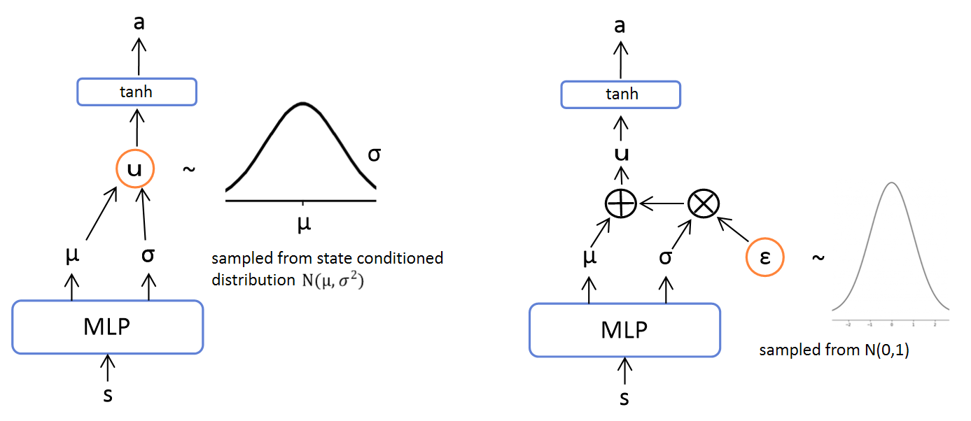
If we sample actions as the left graph does, the backpropagation of the objective will be stopped at the sampling node. Therefore, by separating the sampling node as the right graph does, we can use backpropagation to update the policy parameters \(\phi\). Now, we can rewrite the objective in Equation \ref{eqn:policy-obj} as
\[\begin{equation} J_\pi(\phi) = \mathbb E_{s_t \sim \mathcal D, \epsilon \sim \mathcal N} \left[ \mathrm{log} \ \pi_\phi(f_\phi(\epsilon_t;s_t) \mid s_t) - \underset{ i \in \left\lbrace 1,2 \right\rbrace }{\mathrm{min}} \ Q_{\theta_i}(s_t,f_\phi(\epsilon_t;s_t)) \right], \end{equation}\]which can be optimized with unbiased gradient estimator
\[\begin{equation} \hat{\nabla}_ \phi J_\pi(\phi) = \nabla_ \phi \mathrm{log} \ \pi_\phi(a_t \mid s_t) + \left( \nabla_ {a_t} \mathrm{log} \ \pi_\phi (a_t \mid s_t) - \nabla_ {a_t} \underset{ i \in \left\lbrace 1,2 \right\rbrace }{\mathrm{min}} \ Q_{\theta_i}(s_t,a_t) \right) \nabla_ \phi f_\phi(\epsilon_t;s_t), \end{equation}\]where \(a_t\) is evaluated at \(f_\phi(\epsilon_t;s_t)\).
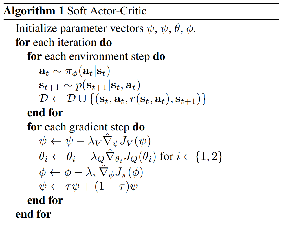
The complete algorithm is described in Algorithm 1.
Experiments
The goal of experimental evaluation is comparing the sample complexity and stability of SAC with prior on/off-policy deep RL algorithms on continuous control tasks. DDPG, PPO, SQL, and TD3 are used for comparison, where exploration noise of DDPG and PPO is turned off and only the mean action for SAC is used in evaluation rollouts. (remove any stochasticity and noise of algorithm in order for the algorithms can fully exploit their knowledge)
Comparative Evaluation
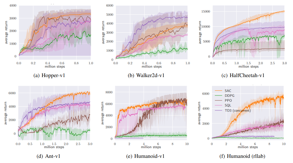
SAC performs comparably to the baseline methods on the easier tasks and outperforms them on the harder tasks with a large margin, both in terms of learning speed(vs. PPO, SQL especially) and the final performance(vs. DDPG, SQL especially).
Ablation study
To check which particular components of SAC are important for good performance and how sensitive SAC is to some of the most important hyperparameters.
1. Stochastic vs. deterministic policy
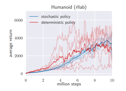
Comparison of SAC and a deterministic variant of SAC (closely resembles DDPG, with the exception of 2 Q-func., hard target updates, no target actor, fixed exploration noise) shows that learning a stochastic policy with entropy maximization can drastically stabilize training.
2. Policy evaluation
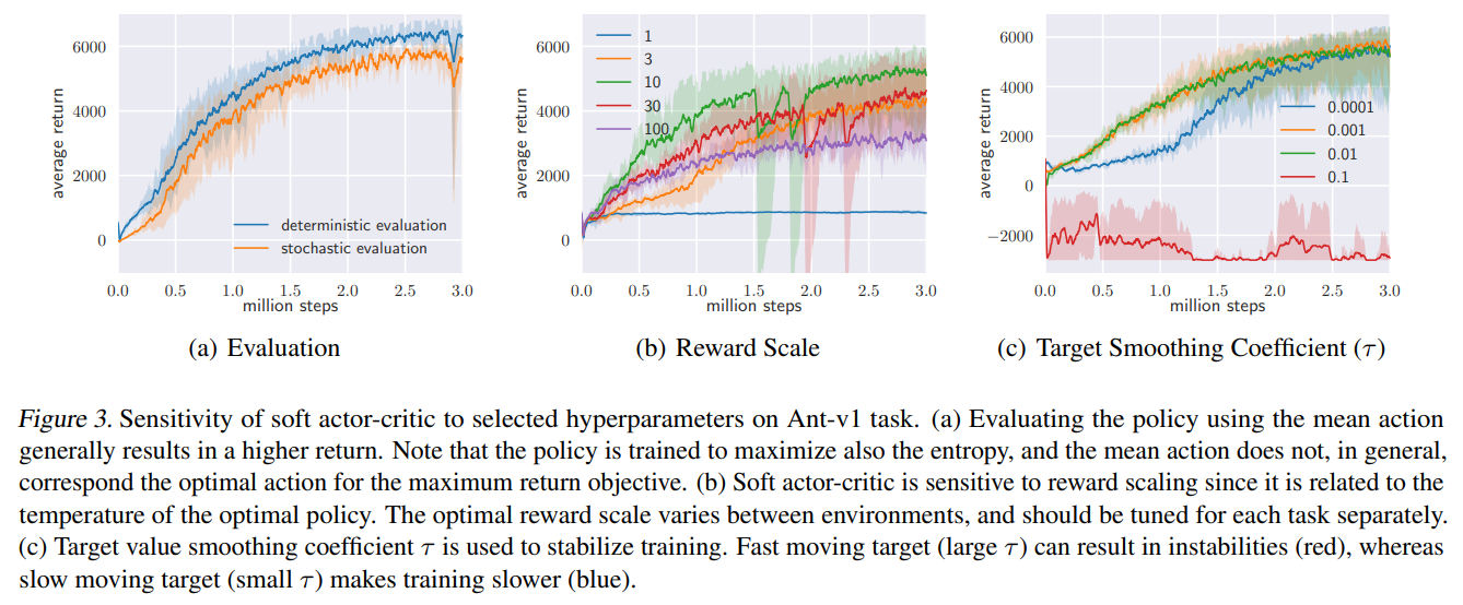
Deterministic evaluation (choosing the mean of the policy distribution at evaluation rollouts) can yield better performance than stochastic evaluation.
3. Reward scale
Soft actor-critic is particularly sensitive to the scaling of the reward signal, because it serves the role of the temperature of the energy-based optimal policy (\(\propto 1/\alpha\)) and thus controls its stochasticity.
| Reward magnitudes | Policy | Problem |
|---|---|---|
| Small | nearly uniform | fail to exploit the reward signal |
| Large | nearly deterministic | lack of adequate exploration |
They found that reward scale to be the only hyperparameter that requires tuning. The need of manual hyperparameter tuning leads to the follow up study of Automating Entropy Adjustment for Maximum Entropy RL.
4. Target network update
Using a separate target value network that slowly tracks the actual value function improves stability. They found that the range of suitable values of \(\tau\) to be relatively wide.
The results of experiment 2 - 4 are described below.
