MPC-PEARL
TL;DR:
- MPC-PEARL: a novel combination of meta-RL and MPC with event-triggered probabilistic switching between the two modules.
- Event-triggered switching makes up for ineffective behaviors of PEARL with MPC, encouraging exploration of potentially high-reward regions.
- Randomization layer induces MPC-PEARL to learn frequently from actions generated by MPC, thereby complementing suboptimal MPC actions caused by the limited prediction horizon.
- GPR and CVaR constraint are used in MPC to build safe region constraint with unknown motion of dynamic obstacles.
- An online adaptdation scheme enables the robot to infer and adapt to a new task within a single trajectory.
Introduction
Limitations of meta-RL & MPC
As it is crucial for mobile robots to adapt quickly to environmental changes, meta-RL algorithms (e.g. PEARL) are suitable for robot navigation problems. However, the meta-learned policy may be conservative in some situations. Another sequential decision-making tool, which is MPC, can be used to infer unknown parts of the system or environmental model with various ML techniques. But, learning-based MPC techniques are computationally demanding and MPC optimizes an action sequence within a fixed short horizon, causing suboptimal, myopic behaviors in general.
Motivation of MPC-PEARL
There have been a few attemps to use MPC in model-based meta-RL or meta-learning methods, such as using learned MPC in real-time decision making. However, none of them utilizes the actions generated by MPC in the training stage. Motivated by this observation, the authors proposed a systematic approach to infusing MPC into the meta-RL training process for mobile robots in environments cluttered with moving obstacles.
Preliminaries
Motion Control in Dynamic Environments
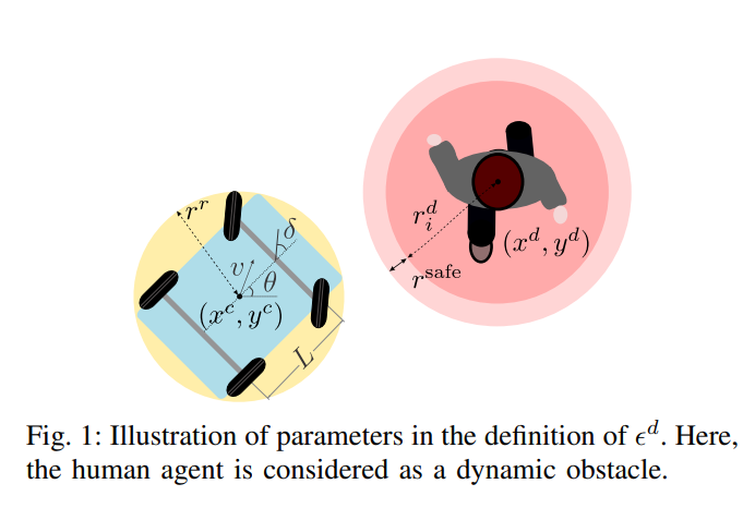
The motions of the robot and obstacles
-
The motion of the robot is modeled by the following discrete-time nonlinear system:
\(\begin{equation}\label{eqn:robot-motion} x_{t+1} = f(x_t, u_t), \end{equation}\) where \(x_t \in \mathcal X \subseteq \mathbb R^{n_x}\) and \(u_t \in \mathcal U \subseteq \mathbb R^{n_u}\) are the robot’s state and control input at stage t.
- state of dynamic obstacles: \(x_{t,i}^d \in \mathbb R^{n_d}, i=1, ..., N_d\)
- state of static obstacles: \(x_i^s \in \mathbb R^{n_s}, i=1,...,N_s\)
- As a common practice, the obstacles’ motion can be tracked with high accuracy (fully observability assumption).
Definition of the motion control problem
- The motion control problem: MDP tuple \(\mathcal T := \left( \mathcal{S,U} , P, c, \gamma \right)\) , where \(\mathcal S \subseteq \mathbb R^{n_x+n_dN_d+n_sN_s}\) and \(\mathcal U\) are the state and action spaces, respectively, \(c\) iis a stage-wise cost function of interest.
- The MDP state: \(s_t := \left( x_t,x_{t,1}^d, ..., x_{t,N_d}^d, x_1^s,..., x_{N_s}^s \right)\) , concatenating the robot state and the states of the static and dynamic obstacles.
-
The stage-cost function \(c\) is chosen as follows:
\[\begin{equation}\label{eqn:cost} c(s_t,u_t) := l(x_t,u_t) + w_d \mathbf 1_{ \lbrace x_t \notin \mathcal X_t^d \rbrace } + w_s \mathbf 1_{ \lbrace x_t \notin \mathcal X^s \rbrace } - w_g \mathbf 1_{ \lbrace x_t \in \mathcal X^g \rbrace } , \end{equation}\]where the loss function \(l\) measures the control performance, \(\mathcal X_t^d\) and \(\mathcal X^s\) denote the safe regions with respect to dynamic and static obstacles to be defined.
- \(\mathcal X_t^d := \lbrace x \in \mathbb R^{n_x} \mid h_d(x,x_{t,i}^d) \geq \epsilon_i^d, i=1,...N_d \rbrace\) : The safety function is \(h_d(x,x_i^d) := \lVert p^r -p_i^d \rVert_2\) , where \(p^r\) and \(p_i^d\) represent the center of gravities of the robot and dynamic obstacle \(i\) , respectively. The threshold is \(\epsilon_i^d = r^r+r_i^d+r^\text{safe}\) , where \(r^r\) and \(r_i^d\) are the radii of balls covering the robot and the obstacle respectively. \(\mathcal X^s\) can be designed in a similar manner.
- \(\mathcal X^g := \lbrace x \in \mathbb R^{n_x} \mid \lVert p^r -p_\text{goal} \rVert_2 \leq \epsilon^g \rbrace\) : incentivizes the robot to reach a neighborhood of the goal point.
Off-Policy Meta-Reinforcement Learning
As the motion pattern of dynamic obstacles and the configuration of static obstacles (transition function \(P\) and cost function \(c\) ) vary, it is desired to train the robot via meta-RL. To enhance sample efficiency in meta-RL, adopt PEARL, which is a state-of-the-art off-policy meta-RL algorithm. (You can see detailed explanations on PEARL algorithm at the link above.)
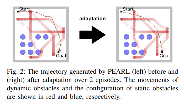
Fig. 2 shows how the PEARL policy operates in the robot navigation task. This example indicates that PEARL policies may induce overly conservative behaviors to bypass regions cluttered with moving obstacles.
Infusing MPC into Meta-RL
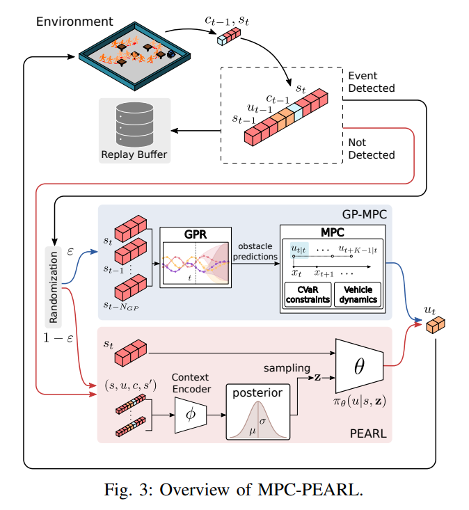
To resolve the limited nagivation performance of PEARL, learning-based MPC is combined to provide it with transition samples in case a predefined event occurs. (The authors considered the following two events that are ineffectively handled by PEARL: (Event 1) collision with a dynamic obstacle, and (Event 2) reaching the neighboring region of the goal point.) If the MPC module is activated, a carefully designed MPC problem is solved using GPR result of inferring the motion of obstacles. Otherwise, the original PEARL algorithm chooses an action. Note that the randomization layer induces MPC-PEARL to learn frequently from actions generated by MPC.
MPC-PEARL Algorithm
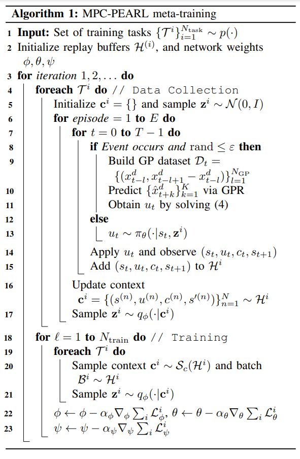
- (line 4-17) Transition samples are collected for each task \(\mathcal T^i\) to build a task-specific replay-buffer \(\mathcal H^i\) .
- (line 9-11) A carefully designed MPC predicts the motion of dynamic obstacles via GPR and to avoid collisions via CVaR constraints.
- (line 20) \(\mathcal S_c\) is chosen to generate transition samples uniformly from the most recent data collection stage.
- (line 22-23) The policy is trained using
soft actor-critic (SAC)and the context encoder network is trained as inPEARL.
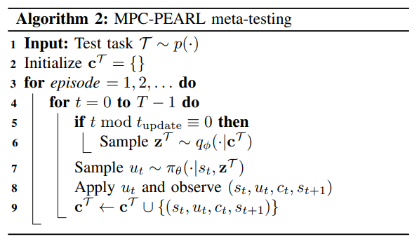
- By omitting the MPC module during meta-testing, a significant amount of computation time can be saved.
- (line 5-6) The online adaptation scheme, performed within a single trajectory, is crucial for some practical applications where each episode is less likely to be repeated due to its consistently evolving environments.
Learning-Based MPC with CVaR Constraints
As PEARL does not use the known system dynamcis that is often available for various practical robots, authors adpoted a learning-based MPC technique that solves the given task and uses model information in a receding horizon fashion:
\[\begin{align}\label{eqn:MPC-det} \begin{split} \underset{\mathbf u}{\mathrm{min}}\ & J(x_t, \mathbf u) = l_f(x_{t+K \mid t} ) + \sum_{k=0}^{K-1} l(x_{t+k \mid t} , u_{t+k \mid t} ) \\ \text{s.t.}\ & x_{t+k+1 \mid t} = f(x_{t+K \mid t} , u_{t+k \mid t}) \\ & x_{t \mid t} = x_t \\ & x_{t+k \mid t} \in \mathcal X_{t+k}^d \cap \mathcal X^s \\ & u_{u+k \mid t} \in \mathcal U, \end{split} \end{align}\]where \(\mathbf u = (u_{t \mid t} , ... , u_{t+K-1 \mid t} )\) is a control sequence over the \(K\) prediction horizon, (3b) and (3e) must be satisfied for \(k=0,..., K-1\) and (3d) (safe region constraint) must hold for \(k=0,...K\) . Unfortunately, the MPC problem in the above form is impossible to solve because in general the safe region \(\mathcal X_{t+k}^d\) is unknown; it includes information about the future motion of dynamic obstacles. Here are how the authors solved this problem.
Learning the motion of obstacles via GPR (What is GPR?)
- GPR is performed online using a training dataset \(\mathcal D_t = \lbrace x_{t-l}^d, v_{t-l}^d \rbrace_{l=1}^{N_\mathrm{GP}} = \lbrace \tilde{\mathrm{x}}, \tilde{\mathrm{v}} \rbrace\) (\(N_\mathrm{GP}\) most recent observations of the obstacles’ state transitions), where \(v_{t-l}^d := x_{t-l+1}^d - x_{t-l}^d\) .
-
The GPR problem is defined for each \(j\) th entry of \(\mathbf v\) as
\[\begin{align*} \ \ \tilde{\mathrm{v}}_ j = & \mathbf{v}_ j (\tilde{\mathrm{x}}_ j) + \omega_j.\\ \text{where} \ \ & \mathbf{v}_ j (\mathrm{x}) \sim \mathcal{GP}(\mathbf{0}, k_j(\mathrm{x, x'})) \\ & k_j(\mathrm{x,x'}) = \sigma_f^2 \ \mathrm{exp} \left( - \frac{ \lVert \mathrm{x}_ j - \mathrm{x_j'} \rVert }{2\lambda^2} \right) \\ & \omega_j \sim \mathcal N \left( \mathbf{0}, \text{diag} \left[ \sigma_{\omega, j}^2, \ldots , \sigma_{\omega, j}^2 \right] \right) \end{align*}\] -
The corresponding approximation of \(\mathbf v\) at an arbitrary test point \(\mathbf x\) is then represented by \(\mathbf v(\mathbf x) \sim \mathcal N (\mu^v(\mathbf x), \Sigma^v(\mathbf x))\) , where \(\mu^v\) and \(\Sigma^v\) are computed as
\[\begin{align*} \mu_j^v(\mathbf x) &= K_j(\mathbf x, \tilde{\mathrm{x}}) \left[ K_j(\tilde{\mathrm{x}}, \tilde{\mathrm{x}}) + \sigma_{\omega, j}^2 I \right]^{-1} \tilde{\mathrm{v}}_ j \\ \Sigma_j^v(\mathbf x) &= k_j(\mathbf{x, x}) - K_j(\mathbf x, \tilde{\mathrm{x}}) \left[ K_j(\tilde{\mathrm{x}}, \tilde{\mathrm{x}}) + \sigma_{\omega, j}^2 I \right]^{-1} K_j(\tilde{\mathrm{x}}, \mathbf x) \end{align*}\] -
Starting from \(\hat{x}_ t^d \sim \mathcal N(x_t^d, \mathbf 0)\) , the approximated state of the obstacle \(\hat{x}_ {t+k+1}^d \sim \mathcal N(\mu_{t+k+1}, \Sigma_{t+k+1})\) is obtained by propagating the state vector using the estimated velocity evaluated at the current mean state:
\[\mu_{t+k+1} = \mu_{t+k} + \mu^v(\mu_{t+k}), \ \ \Sigma_{t+k+1} = \Sigma_{t+k} + \Sigma^v(\mu_{t+k})\]
CVaR constraints for safety
- Due to the stochastic nature of \(\hat{\mathcal X}_ {t+k}^d\) , imposing the deterministic constraint \(x_{t+k \mid t} \in \hat{\mathcal X}_ {t+k}^d\) is likely to cause infeasibility or an overly conservative solution.
- As a remedy a probabilistic constraint is used: CVaR constraint
- CVaR of a random loss \(X\) is its expected value within the \((1-\alpha)\) worst-case quantile and is defined as \(\mathrm{CVaR}_ \alpha [X]:= \mathrm{min}_ {\xi \in \mathbb R} \mathbb E [\xi + (X - \xi)^+ / (1 -\alpha)]\) , where \(\alpha \in (0,1)\) and \((x)^+ = \mathrm{max} \lbrace x,0 \rbrace\) (Check
Conditional Value-at-Risk (CVAR): Algorithms and Applicationsby Stan Uryasev if you want more detailed explanations. - CVaR is a convex risk measure and discerns a rare but catastrophic event in the worst-case tail distribution unlike chance constraits. (As CVaR is a expectation value)
-
By replacing a random loss \(X\) in CVaR definition with \(L(x_t, \hat{x}_ t^d) := \mathrm{max}_ {i=1,...N_d} \lbrace \epsilon_i^d - h_d(x_t,\hat{x}_ {t,i}^d) \rbrace\) , the deterministic safe region constrint (3d) now can be written in probabilistic as
\[\mathrm{CVaR}_ \alpha \left[ L(x_{t+k \mid t}, \hat{x}_ {t+k}^d) \right] = \underset{\xi \in \mathbb R}{\mathrm{min}} \left( \xi + \frac{1}{1-\alpha} \mathbb E \left[ \left( L(x_{t+k \mid t}, \hat{x}_ {t+k}^d) - \xi \right)^+ \right] \right) \leq \delta_{\text{CVaR}},\]where \(\delta_\text{CVaR}\) is a user-specific non-negative threshold representing the maximum tolerable risk level.
-
CVaR constraint can be approximated by sample average approximation (SAA) using a GPR distribution samples \(\lbrace \hat{x}_ {t+k}^{d, (m)} \rbrace_{m=1}^{M_\mathrm{SAA}}\) . The resulting GP-MPC formulation is
\[\begin{align} \begin{split} \underset{\mathbf u, \xi}{\mathrm{min}}\ & J(x_t, \mathbf u) \\ \text{s.t.}\ & \xi_k + \sum_{m=1}^{M_\text{SAA}} \frac{ \left(L(x_{t+k \mid t}, \hat{x}_ {t+k}^{d,(m)}) - \xi_k \right)^+}{M_{\text{SAA}}(1-\alpha)} \leq \delta_\text{CVaR} \\ & x_{t+k \mid t} \in \mathcal X^s \\ & (3b), (3c), \text{and} (3e). \end{split} \end{align}\]
Simulation Results
Simulation Details
Robot Dynamics
- state: the robot’s CoG \((x_t^c, y_t^c)\) and the heading angle \(\theta_t\)
- control input (available action): the velocity \(v_t\) and the steering angle of the front wheel \(\delta_t\) , where the action space is set to \(\mathcal U:= [9,v_\text{max}] \times [-\frac{\pi}{2}, \frac{\pi}{2}]\) .
- The transition model of robot in \eqref{eqn:robot-motion} are now given by
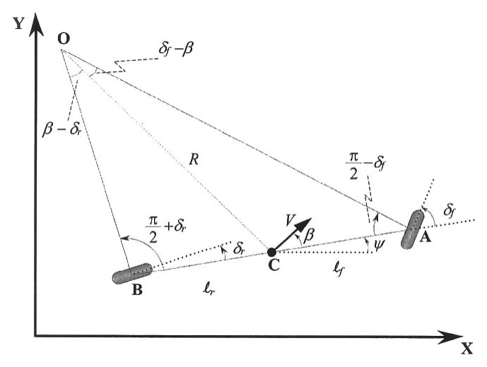
where \(T_s\) is the sample time and the slip angle \(\beta_t\) is defined as \(\beta_t := \mathrm{tan}^{-1}(\frac{\mathrm{tan} \delta_t}{2})\) .
MPC-PEARL Details
- The MPC module is activated with a probability of \(\epsilon \in \lbrace 0.2, 0.5, 0.8, 1 \rbrace\) when the event occur.
- The loss function in \eqref{eqn:cost} is chosen to speed up navigation with limited control energy as \(l(x_t, u_t) := \lVert x_t - x_\text{goal} \rVert_Q^2 + \lVert u_t \rVert_R^2\) where \(Q =\mathrm{diag}[1,1,0], R=0.2I_{n_u}\) .
- The terminal cost function in \eqref{eqn:MPC-det} was chosen similarly to the loss function in the cost function as \(l_f(x) := \lVert x-x_\text{goal} \rVert_{Q_f}^2\) with \(Q_f = 20 Q\) .
- The GPR is performed using the latest \(N_\text{GP} = 10\) observations for predicting the motion of the closest \(N_\text{adapt} = 2\) obstacles for a planning horizon of \(K = 10\) .
Baseline Algorithms and Performance Metrics
MPC-PEARL is compared to PEARL, GP-MPC, MPC-SAC and GRBAL (Model-based meta-RL method with gradient-based MAML), using the following metrics:
- Success Rate (SR): reaching the goal point & no collision occurs
- Travel Time (TT): time to reach the goal without any collision
- Collision-Free Rate (CFR): # no collision tasks / # all tasks
- Success Weighted by Path Length (SPL): \(\frac{1}{N} \sum_{i=1}^N S_i \frac{l_i}{\mathrm{max}}(p_i, l_i)\) where \(l_i\) is the shortest-path distance from the agent’s starting position to the goal in episode i, \(p_i\) is the length of path actually taken by agent and \(S_i\) is a binary indicator of success in episode i.
- Mean Goal Distance (MGD): the average euclidean distance between the robot and the goal
Restaurant Environment
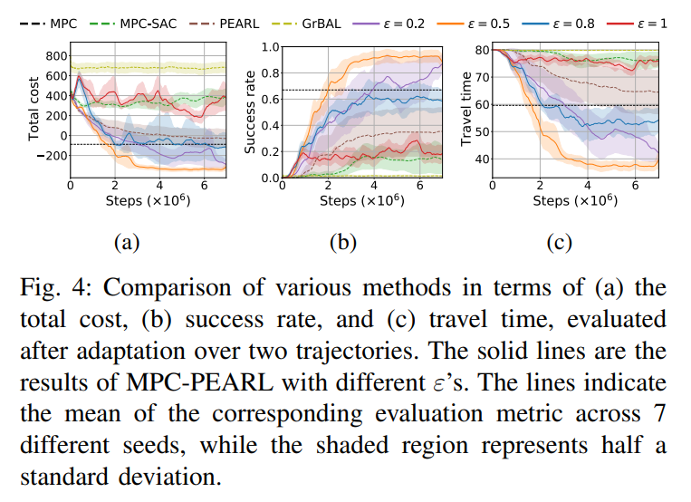
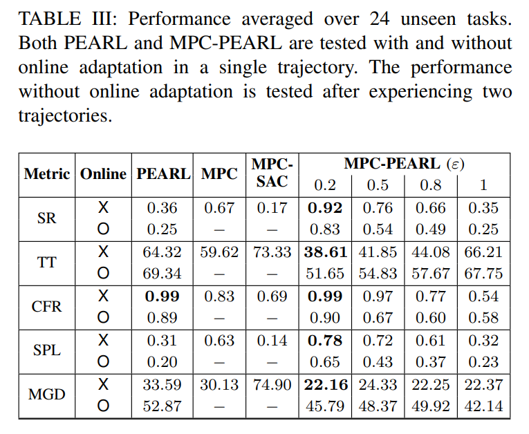
- Fig. 4 displays that MPC-PEARL with \(\epsilon = 0.2, 0.5\) shows the best performance not the case with \(\epsilon = 0.8\) or \(1\) , which has fewer opportunities to discover control actions that are better than MPC actions. This indicates that MPC-PEARL effectively exploits both MPC and PEARL to attain better navigation performances.
- GrBAL presents the worst performance in terms of all metrics. As GrBAL is a pure model-based method, it suffers from the bias accumulated during trajectory rollouts. Also, the lack of a systematic exploration scheme degrades the overall performance.
- The systematic infusion of MPC actions accelerates meta-training, particularly in the early stages. However, the infusion rate should be kept under a certain threshold to improve the overall performance.
- The online adaptation scheme does not significantly degrade the performance of the MPC-PEARL policy with \(\epsilon = 0.2\) although the online version uses much less information.
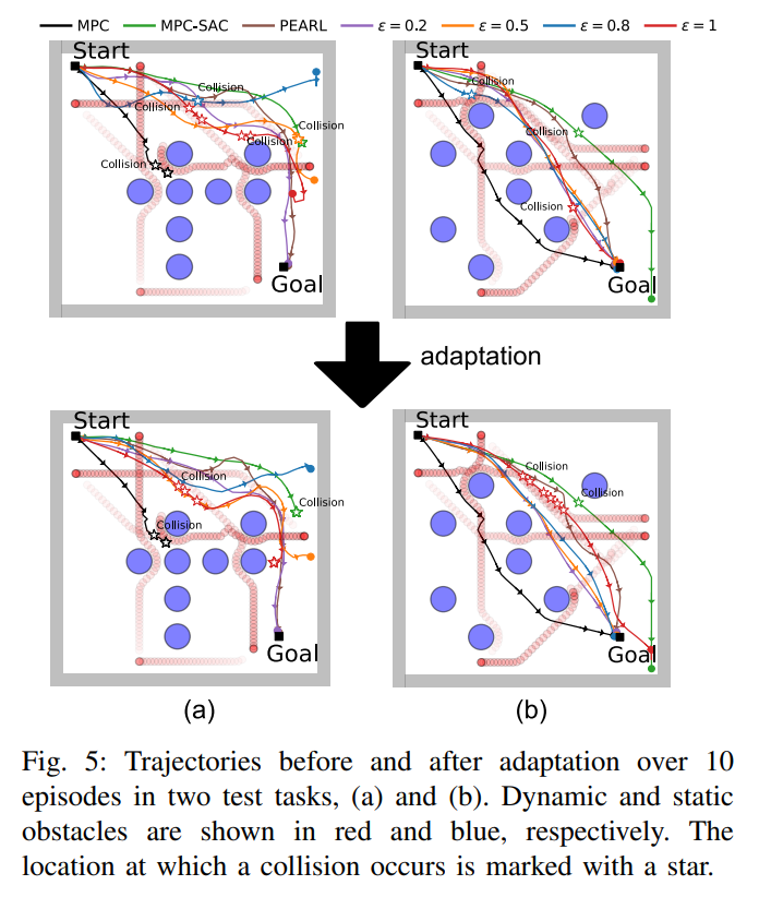
- In Fig. 5 (a), the robot controlled by MPC is stuck in the middle due to its short horizon.
- In Fig. 5 (b), PEARL steers the robot toward a conservative path, detouring the cluttered region.
- In the case of MPC-PEARL with \(\epsilon = 0.2, 0.5, 0.8\) , the robot takes a riskier yet shorter path without a collision.
Sidewalk Environment
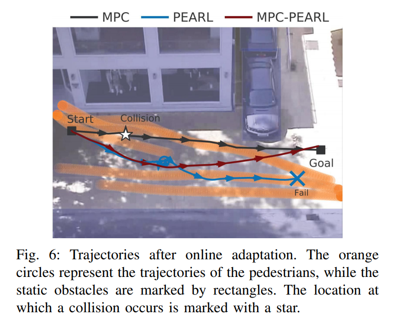
- The agressive goal-oriented nature of GP-MPC causes a collision (SR:0.48, TT:59.62).
- PEARL displays a conservative behavior that does not lead to any collisions (CFR:0.84), but falling behind GP-MPC in terms of navigation performance (SR:0.03, SPL: 0.03, TT:249.61).
- MPC-PEARL with \(\epsilon = 0.2\) showed the best performance, balancing safety and efficiency (SR:0.67, TT:211.35, SPL:0.44).