MBMRL for Flight
TL;DR:
- Proposed a meta-learning approach that “learns how to learn” models of various payloads that a priori unknown physical properties vary dynamics.
- By augmenting the dynamic model with stochastic latent variables, the authors infused meta-learning approach into MBRL.
- Usage of unknown latent variables leads to outperforming results compared to pure model-based methods.
- By online adaptation mechanism, the dynamics variables converges and the tracking error also reduces.
- Proposed approach shows improved performance for the full end-to-end payload trasportation task as well as transporting a suspended payload towards a moving target, around an obstacle by following a predefined path, and along trajectories dictated using a “wand”-like interface.
Introduction
Task definition

Limits of hand-designed model on the flight tasks
The complex interaction between the magnetic gripper and the payload are unlikely to be represented accurately by hand-designed models. Even more unpredictable is the effect of the payload on the dynamics of the quadcopter when the payload is lifted off the ground.
Need for fast adaptation
Conventional learning-based methods typically require a large amount of data to learn accurate models, and therefore may be slow to adapt. The payload adaptation task illustrates the need for fast adaptation; the robot must very quickly determine the payload parameters, and then adjust its motor commands accordingly.
Proposed method: model-based meta-RL
A predictive dynamics model which is augmented with stochastic latent variables is learned with different payload masses and tether lengths. In test time, it uses variational inference to estimate the corresponding posterior distribution over these latent variables.
Related Work
Controlling Aerial Vehicles
- Prior works on control for aerial vehicles that relying on manual system identification : require a priori knowledge of the system
- Automating system identification via online parameter adaptation : still rely on domain knowledge for the equations of motion
- Adaptive model-based controller : require a priori knowledge of dynamic systems, parameters for state estimation, etc.
- In contrast, the proposed data-driven method only requires the pixel location of the payload and the quadrotor’s commanded actions to control and adapt to the suspended payload’s dynamics.
End-to-end Learning-based Approach
- The learning processes of value-based and gradient-based methods generally take hours or even days, making it poorly suited for safety-critical and resource-constrained quadcopters.
- Model-based reinforcement learning (MBRL) can provide better sample efficiency, but must MBRL methods are designed to model a single task with unchanging dynamics, and therefore do not adapt to rapid online changes in the system dynamics.
Model-based Meta-learning
-
O'Connell et al.used MAML algorithm for adapting a drone’s internal dynamics model. The resulting adapted model, however, did not improve the performance of the closed-loop controller. In contrast, the authors demonstrate that their method does improve performance of the model-based controller. -
Nagabandi et al.(GrBAL)andKaushik et al.explored meta-learning for online adaptation in MBRL for a legged robot, which demonstrated improved closed-loop controller performance with adapted model.
Preliminaries: PETS Algorithm
Model-based reinforcement learning estimates the underlying dynamics from data by training a dynamics model \(p_\theta(s_{t+1} \mid s_t, a_t)\) via maximum likelihood
\[\begin{align} \theta^* &= \underset{\theta}{\mathrm{argmax}} \ p(\mathcal D^\text{train} \mid \theta) \nonumber\\ \label{eqn:model-train} &= \underset{\theta}{\mathrm{argmax}} \sum_{(s_t,a_t,s_{t+1}) \in \mathcal D^\text{train}} \mathrm{log} \ p_\theta(s_{t+1} \mid s_t, a_t). \end{align}\]To instantiate this method, the authors extend the PETS algorithm, which handles expressive neural network dynamics models to attain good sample efficiency as model-based algorithms and asymptotic performance as model-free algorithms.
Probabilistic ensemble NN
Why ‘Probabilistic NN’ and ‘Ensemble of NNs’?
- The capacity of model is a critical ingredient in the asymptotic performance of MBRL methods
- NN models can scale to large datasets, however, NNs tend to overfit on small datasets.
- This issue can be mitigated by properly incorporating uncertainty into the dynamics model -> Probailistic NN !
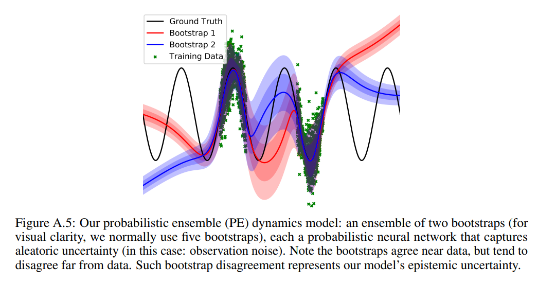
- Two types of uncertainty: (1) aleatoric uncertainty: inherent stochasticities of a system, (2) epistemic uncertainty: subjective uncertainty due to a lack of sufficient data to uniquely determine the underlying system exactly.
- ‘Probabilistic NN’ can capture aleatoric uncertainty and ‘Ensembles’ can capture epistemic uncertainty.
PETS uses an ensemble of probabilistic neural network models, each parameterizing a Gaussian distribution of \(s_{t+1}\) conditioned on both \(s_t\) and \(a_t\) , i.e.: \(\tilde{f} = \mathrm{Pr}(s_{t+1} \mid s_t, a_t) = \mathcal N(\mu_\theta(s_t,a_t), \Sigma_\theta (s_t,a_t))\) . The negative log prediction probability is used for loss function:
\[\begin{align*} \mathrm{loss_P}(\theta) &= - \sum_{n=1}^N \mathrm{log}\ \tilde{f}_ \theta (s_{n+1} \mid s_n, a_n) \\ &= \sum_{n=1}^N \left[ \mu_\theta (s_n,a_n) - s_{n+1} \right]^\top \Sigma_\theta^{-1} (s_n,a_n) \left[ \mu_\theta(s_n,a_n) -s_{n+1} \right] + \mathrm{log}\ \mathrm{det}\ \Sigma_\theta(s_n,a_n). \end{align*}\]Ensembles of B-many bootstrap models, using \(\theta_b\) to refer to the parameters of \(b^\mathrm{th}\) model \(\tilde{f}_ {\theta_b}\) , define predictive probability distributions: \(\tilde{f_\theta} = \frac{1}{B} \sum_{b=1}^B \tilde{f}_ {\theta_b}\) . Each of bootstrap models have their unique dataset \(\mathbb D_b\) , generated by sampling (with replacement) \(N\) times the dynamics dataset recorded so far \(\mathbb D\) , where \(N\) is the size of \(\mathbb D\) . A visual example of ensembles is provided below.
State Propagation via Trajectory Sampling (TS)
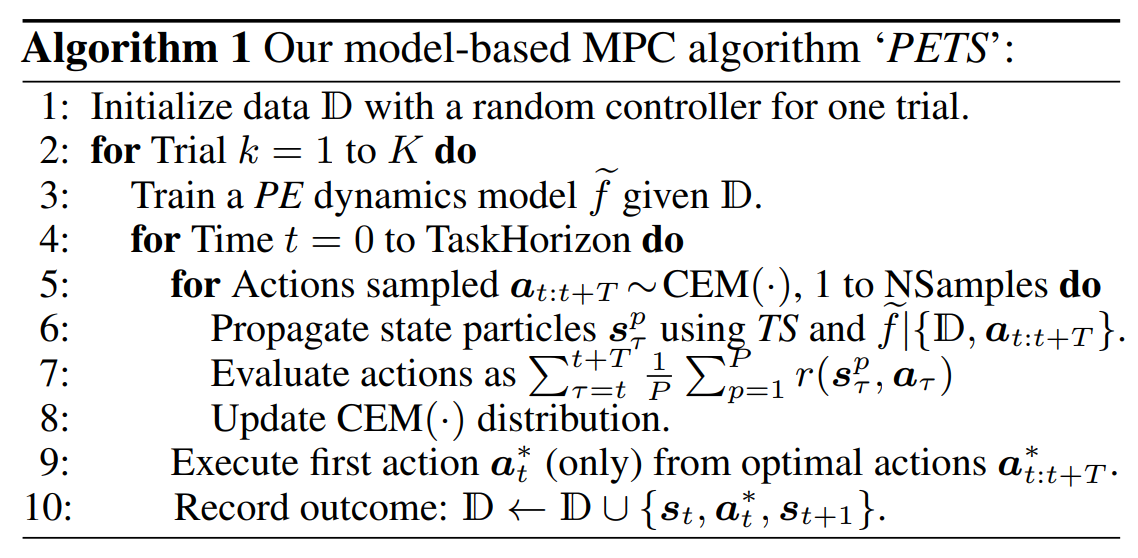
The learned dynamics model is used to plan and execute actions via model predictive control (MPC) with trajectory sampling (TS), since the probabilistic dynamics model \(\tilde{f}\) induces a distribution over the resulting trajectories \(s_{t:t+T}\) for a given control input \(a_{t:t+T} \doteq \lbrace a_t, \ldots , a_{t+T} \rbrace\) . Trajectory sampling predicts plausible state trajectories begins by creating \(P\) particles from the current state, \(s_{t=0}^p =s_0 \ \forall p\) . Each particle is then propagated by: \(s_{t+1}^p \sim \tilde{f}_ {\theta_{b(p,t)}} (s_t^p,a_t)\) , according to a particular bootstrap \(b(p,t)\ \text{in} \lbrace 1, \ldots, B \rbrace\) , where \(B\) is the number of bootstrap models in the ensemble.
Optimizing action sequence via Cross-Entropy Method (CEM)
Unlike a common technique to compute the optimal action sequence (random sampling shooting), PETS used cross-entropy method(CEM). The cross-entropy (CE) method is an adaptive importance sampling procedure for the estimation of rare-event probabilities, which uses the cross-entropy or Kullback-Leibler divergence as a measure of closeness between two sampling distributions. By using the cross-entropy method to gradually change the sampling distribution of the random search so that the rare-event, especially locating an optimal or near optimal solution using naive random search, is more likely to occur. Eventually, the sampling distribution converges to a distribution with a probability mass concentrated in a region of near-optimal solutions.
The CE method can be applied to two types of problems:
- Estimation: Estimate \(l = \mathbb E[H(\mathbf X)]\) , where \(\mathbf X\) is a random object taking values in some set \(\mathfrak X\) and \(H\) is a function on \(\mathfrak X\) . An important special case is the estimation of a probability \(l = \mathbb P(S(\mathbf X) \geqslant \gamma)\) , where \(S\) is another function on \(\mathfrak X\) .
- Optimization: Optimize a given objective function \(S(\mathbf x)\) over all \(\mathbf x \in \mathfrak X\) . \(S\) can be either a known or a noisy function. In the latter case the objective function needs to be estimated, e.g. via simulation.
Cross-Entropy for Rare-event Probability Estimation
Consider the estimation of the probability
\[l = \mathbb P(S(\mathbf X) \geqslant \gamma) = \mathbb E \left[ \mathbf I_{\lbrace S(\mathbf X) \geqslant \gamma \rbrace} \right] = \int \mathbf I_{\lbrace S(\mathbf X) \geqslant \gamma \rbrace} f(\mathbf x ; \mathbf u) \, d\mathbf x ,\]where \(S\) : real-valued function, \(\gamma\) : threshold or level parameter, \(\mathbf X \sim f(\cdot;\mathbf u)\) : pdf parameterized by a finite-dim vector \(\mathbf u\)
Let \(g\) be another pdf s.t. \(g(\mathbf x) = 0 \Rightarrow H(\mathbf x)f(\mathbf x; \mathbf u) = 0 \ \forall \mathbf x\) . Using the pdf \(g\) , we can represent \(l\) as
\[l = \int \frac{f(\mathbf x; \mathbf u) \mathbf I_{\lbrace S(\mathbf x) \geqslant \gamma \rbrace}}{g(\mathbf x)} g(\mathbf x) \, d \mathbf x = \mathbb E \left[ \frac{f(\mathbf X; \mathbf u) \mathbf I_{\lbrace S(\mathbf X) \geqslant \gamma \rbrace}}{g(\mathbf X)} \right] , \quad \mathbf X \sim g .\]With independent random vectors \(\mathbf{X_1, \ldots, X_N} \underset{\mathrm{iid}}{\sim} g\) , then
\[\hat{l} = \frac{1}{N} \sum_{k=1}^N \mathbf I_{\lbrace S(\mathbf X_k) \geqslant \gamma \rbrace} \frac{f(\mathbf X_k;\mathbf u)}{g(\mathbf X_k)}\]is an unbiased estimator of \(l\) : a so-called importance sampling estimator. The optimal importance sampling pdf (that is, the pdf \(g^*\) for which the variance of \(\hat{l}\) is minimal is given as \(g^* (\mathbf x) = f(\mathbf x; \mathbf u) \mathbf I_{\lbrace S(\mathbf x) \geqslant \gamma \rbrace} / l\) . However, as \(l\) is unknown, CE method choose the importance sampling pdf \(g\) from within the parametric class of pdfs \(\lbrace f(\cdot;\mathbf v), \mathbf v \in \mathcal V \rbrace\) s.t. the KL divergence between \(g^*\) and \(g\) is minimal. The CE minimization procedure then reduces to finding an optimal reference parameter vector, \(\mathbf v^*\) say, by cross-entropy minimization:
\[\begin{align*} \mathbf v^* &= \underset{\mathbf v}{\mathrm{argmin}} \mathcal D(g^* , f(\cdot; \mathbf v)) \\ &= \underset{\mathbf v}{\mathrm{argmin}} \int g^* (\mathbf x) \mathrm{ln}\ \frac{g^* (\mathbf x)}{f(\mathbf x;\mathbf v)} \, d \mathbf x \\ &= \underset{\mathbf v}{\mathrm{argmax}} \int g^* (\mathbf x) \mathrm{ln}\ f(\mathbf x;\mathbf v) \, d \mathbf x \\ &= \underset{\mathbf v}{\mathrm{argmax}} \int \frac{f(\mathbf x; \mathbf u) \mathbf I_{\lbrace S(\mathbf x) \geqslant \gamma \rbrace}}{l} \mathrm{ln}\ f(\mathbf x;\mathbf v) \, d \mathbf x \\ &= \underset{\mathbf v}{\mathrm{argmax}} \mathbb E_{\mathbf u} \left[ \mathbf I_{\lbrace S(\mathbf X) \geqslant \gamma \rbrace} \mathrm{ln}\ f(\mathbf X;\mathbf v) \right] \\ &= \underset{\mathbf v}{\mathrm{argmax}} \mathbb E_{\mathbf w} \left[ \mathbf I_{\lbrace S(\mathbf X) \geqslant \gamma \rbrace} \mathrm{ln}\ f(\mathbf X;\mathbf v) \frac{f(\mathbf X;\mathbf u)}{f(\mathbf X;\mathbf w)} \right], \end{align*}\]where \(\mathbf w\) is any reference parameter. This \(\mathbf v^*\) can be estimated via the stochastic sampling:
\[\hat{\mathbf v} = \underset{\mathbf v}{\mathrm{argmax}} = \frac{1}{N} \sum_{k=1}^N \mathbf I_{\lbrace S(\mathbf X_k) \geqslant \gamma \rbrace} \frac{f(\mathbf X_k;\mathbf u)}{f(\mathbf X_k;\mathbf w)} \mathrm{ln}\ f(\mathbf X_k;\mathbf v),\]where \(\mathbf{X_1, \ldots, X_N} \underset{\mathrm{iid}}{\sim} f(\cdot;\mathbf w)\) . The optimal parameter \(\hat{\mathbf v}\) can often be obtained in explicit form, in particular when the class of sampling distributions forms an exponential family.
For a rare-event probability \(l\) , most or all of the indicators \(\mathbf I_{\lbrace S(\mathbf X) \geqslant \gamma \rbrace}\) are zero, and the maximization problem become useless. In that case a multi-level CE procedure is used, where a sequence of reference parameters \(\lbrace \hat{\mathbf v}_ t \rbrace\) and levels \(\lbrace \hat{\gamma}_ t \rbrace\) is constructed with the goal that the former converges to \(\mathbf v^*\) and the latter to \(\gamma\) . The actual procedure is described in the following algorithm.
Algorithm A (CE Algorithm for Rare-Event Estimation) Given the sample size \(N\) and the rarity parameter \(\varrho\) , execute the following steps.
- Define \(\hat{\mathbf v}_ 0 = \mathbf u\) . Let \(N^e = \left \lceil \varrho N \right \rceil\) . Set \(t=1\) (iteration counter).
- Generate \(\mathbf{X_1, \ldots, X_N} \underset{\mathrm{iid}}{\sim} f(\cdot;\hat{\mathbf v}_ {t-1})\) . Calculate \(S_{(i)} = S(\mathbf X_i)\ \forall i\) , and order these from smallest to largest: \(S_{(1)} \leqslant \ldots \leqslant S_{(N)}\) . Let \(\hat{\gamma}_ t\) be the sample \((1-\varrho) \text{-quantile of performances}\) ; that is, \(\hat{\gamma}_ t = S_{(N-N^e+1)}\) . If \(\hat{\gamma}_ t > \gamma\) , reset \(\hat{\gamma}_ t\) to \(\gamma\) .
- Use the same sample \(\mathbf{X_1, \ldots, X_N}\) to solve the stochastic program: \(\hat{\mathbf v}_ t = \underset{\mathbf v}{\mathrm{argmax}} = \frac{1}{N} \sum_{k=1}^N \mathbf I_{\lbrace S(\mathbf X_k) \geqslant \hat{\gamma}_ t \rbrace} \frac{f(\mathbf X_k;\mathbf u)}{f(\mathbf X_k;\hat{\mathbf v}_ {t-1})} \mathrm{ln}\ f(\mathbf X_k;\mathbf v).\)
- If \(\hat{\gamma}_ t < \gamma\) , set \(t = t+1\) and reiterate from Step 2; otherwise, proceed with Step 5.
- Let \(T=t\) be the final iteration counter. Generate \(\mathbf{X_1, \ldots, X_N} \underset{\mathrm{iid}}{\sim} f(\cdot;\hat{\mathbf v}_ T)\) and estimate \(l\) via importance sampling:
Cross-Entropy Method for Optimization
The estimation algorithm above leads naturally to a simple optimization heuristic. Optimization problem can be written, with an assumtion that only one maximizer \(\mathbf x^*\) exists for simplicity, as
\[S(\mathbf x^* ) = \gamma^* = \underset{\mathbf x \in \mathfrak X}{\mathrm{max}}\ S(\mathbf x).\]We can now associate with the above optimization problem the estimation of the probability \(l = \mathbb P(S(\mathbf X) \geqslant \gamma)\) , where \(\gamma\) is close to the unknown \(\gamma^*\) . Typically, \(l\) is a rare-event probability, and the multi-level CE approach of Algorithm A can be used to find an importance sampling distribution that concentrates all its mass in a neighborhood of the point \(\mathbf x^*\) . Sampling from such a distribution thus produces optimal or near-optimal states. Although the final level \(\gamma = \gamma^*\) is generally not known in advance, the CE method for optimization produces a sequence of levels \(\lbrace \hat{\gamma}_ t \rbrace\) and reference parameters \(\lbrace \hat{\mathbf v}_ t \rbrace\) such that ideally the former tends to the optimal \(\gamma^*\) and the latter to the optimal reference vector \(\mathbf v^*\) corresponding to the point mass at \(\mathbf x^*\) .
Algorithm B (CE Algorithm for Optimization)
- Choose an initial parameter vector \(\hat{\mathbf v}_ 0\) . Let \(N^e = \left \lceil \varrho N \right \rceil\) . Set \(t=1\) (level counter).
- Generate \(\mathbf{X_1, \ldots, X_N} \underset{\mathrm{iid}}{\sim} f(\cdot;\hat{\mathbf v}_ {t-1})\) . Calculate the performances \(S_{(i)} = S(\mathbf X_i) \forall i\) , and order them from smallest to largest: \(S_{(1)} \leqslant \ldots \leqslant S_{(N)}\) . Let \(\hat{\gamma}_ t\) be the sample \((1-\varrho) \text{-quantile of performances}\) ; that is, \(\hat{\gamma}_ t = S_{(N-N^e+1)}\) .
- Use the same sample \(\mathbf{X_1, \ldots, X_N}\) to solve the stochastic program: \(\begin{equation} \hat{\mathbf v}_ t = \underset{\mathbf v}{\mathrm{argmax}} = \frac{1}{N} \sum_{k=1}^N \mathbf I_{\lbrace S(\mathbf X_k) \geqslant \hat{\gamma}_ t \rbrace} \mathrm{ln}\ f(\mathbf X_k;\mathbf v). \end{equation}\)
- If some stopping criterion is met, stop; otherwise set \(t=t+1\) , and return to Step 2.
Note that the estimation Step 5 of Algorithm A is missing in Algorithm B, because in the optimization setting we are not interested in estimating \(l\) per se. For the same reason the likelihood ration term \(f(\mathbf X_k;\mathbf u) / f(\mathbf X_k;\hat{\mathbf v}_ {t-1})\) in Algorithm A is missing in Algorithm B. To run the algorithm, (1) a class of parametric sampling densities \(\lbrace f(\cdot;\mathbf v), \ \mathbf v \in \mathcal V \rbrace\) , (2) the initial vector \(\hat{\mathbf v}_ 0\) , (3) the sample size \(N\) , (4) the rarity parameter \(\varrho\) , and (5) a stopping criterion are needed to be predefined.
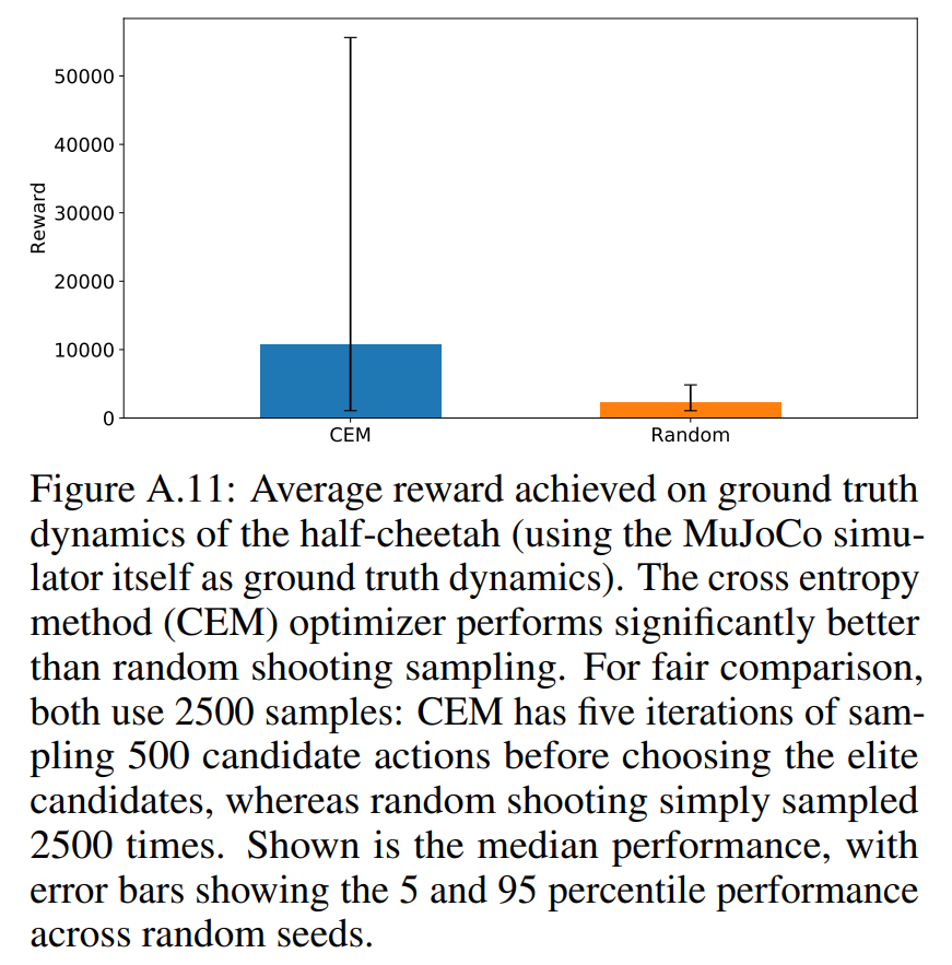
The results from PETS paper show that using CEM significantly outperforms random search on the half-cheetah task. Simple random search techniques are simple and have ease of parallelism, but they suffer in high dimensional spaces.
PETS algorithm summary
Now the overall PETS algorithm can be summarized in Algorithm 1.
Model-Based Meta-Learning For Quadcopter Payload Transport
Data Collection
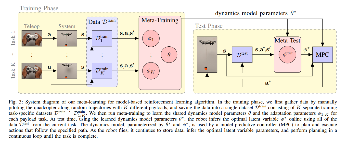
Data is collected by manually piloting the quadcopter along random paths for each of the \(K\) suspended payloads. A dataset \(\mathcal D^\text{train}\) consists of \(K\) separate datasets \(\mathcal D^\text{train} \doteq \mathcal D^\text{train}_ {1:K} \doteq \lbrace \mathcal D^\text{train}_ 1, \ldots , \mathcal D^\text{train}_ K \rbrace\) , one per payload task.
Model Training with Known Dynamics Variables
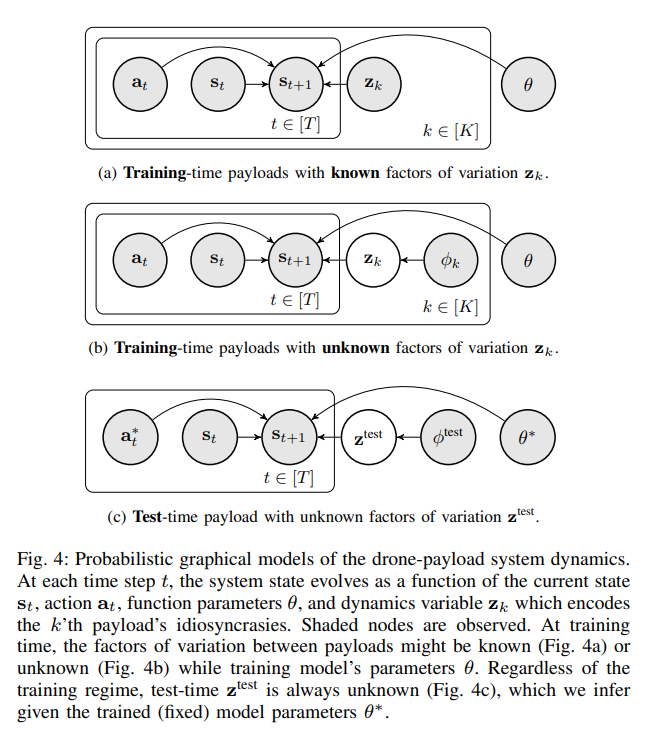
In case we know all the “factors of variation” in the dynamics across tasks at training time, represented explicitly as a “dynamic variable” \(z_k \in \mathbb R^{d_z}\) , we can learn a single dynamics model \(p_\theta\) across all tasks by using \(z_k\) as an auxiliary input to PETS:
\[\begin{equation} s_{t+1} \sim p_\theta (s_{t+1} \mid s_t, a_t, z_k ). \end{equation}\]Training is analogous to \eqref{eqn:model-train} , but with an additional conditioning on \(z_{1:K} \doteq [ z_1, \ldots, z_K ]\) :
\[\begin{align} \theta^* &= \underset{\theta}{\mathrm{argmax}} \ p(\mathcal D^\text{train} \mid z_{1:K}, \theta) \nonumber\\ \label{eqn:known-model-train} &= \underset{\theta}{\mathrm{argmax}} \sum_{k=1}^K \sum_{(s_t,a_t,s_{t+1}) \in \mathcal D^\text{train}_ k} \mathrm{log} \ p_\theta(s_{t+1} \mid s_t, a_t, z_k). \end{align}\]
Meta-Training with Latent Dynamics Variables
In most cases, we can’t know or measure dynamic factors at every training time. Thus, a more general training procedure that infers the dynamics variables \(z_{1:K}\) and the model parameters \(\theta\) jointly. This is begun by placing a prior over \(z_{1:K} \sim p(z_{1:K}) = \mathcal N(0,I)\) , and then jointly infer the posterior \(p(\theta, z_{1:K} \mid \mathcal D^\text{train}_ {1:K} )\) .
Unfortunately, inferring \(p(\theta, z_{1:K} \mid \mathcal D^\text{train}_ {1:K} )\) exactly is computationally intractable. Therefore, the authors used an approximate variational posterior, which is a Gaussian with diagonal covariance, factored over tasks,
\[\begin{equation} q_{\phi_k} (z_k) = \mathcal N(\mu_k, \Sigma_k) \approx p(z_k \mid \mathcal D^\text{train}) \quad \forall k \in [K], \end{equation}\]and parameterized by \(\phi_k \doteq \lbrace \mu_k, \Sigma_k \rbrace\) . Unlike the case of known dynamics variables \eqref{eqn:known-model-train}, now we must marginalize out \(z_{1:K}\) because it is unknown. Therfore, the model training with latent dynamics variables can be written as:
\[\begin{align} \mathrm{log}\ p(\mathcal D^\text{train} & \mid \theta) = \mathrm{log} \int_{z_{1:K}} p(\mathcal D^\text{train} \mid z_{1:K}, \theta) p(z_{1:K})\, dz_{1:K} \nonumber\\ &= \sum_{k=1}^K \mathrm{log}\ \mathbb E_{z_k \sim q_{\phi_k}} p(\mathcal D^\text{train} \mid z_{1:K}, \theta) \cdot p(z_{1:K})/q_{\phi_k}(z_k) \nonumber\\ &\geq \sum_{k=1}^K \mathbb E_{z_k \sim q_{\phi_k}} \sum_{(s_t,a_t,s_{t+1}) \in \mathcal D^\text{train}_ k} \mathrm{log}\ p_\theta(s_{t+1} \mid s_t, a_t, z_k) - \mathrm{KL}(q_{\phi_k}(z_k) \parallel p(z_k)) \quad (\because \text{def. of KL-div & } 0 \leq q \leq 1 \to \text{inequality holds)} \nonumber\\ \label{eqn:marginalize-latent} &\doteq \mathrm{ELBO}(\mathcal D^\text{train} \mid \theta, \phi_{1:K}) . \end{align}\]The propsoed meta-training algorithm then optimizes both \(\theta\) and the variational parameters \(\phi_{1:K}\) of each task with respect to the evidence lower bound
\[\begin{equation}\label{eqn:unknown-model-train} \theta^* \doteq \underset{\theta}{\mathrm{argmax}}\ \underset{\phi_{1:K}}{\mathrm{max}}\ \mathrm{ELBO}(\mathcal D^\text{train} \mid \theta, \phi_{1:K}). \end{equation}\]
Test-Time Task Inference
At test time, the robot must infer the unknown dynamics variables \(z^\text{test}\) online in order to improve the learned dynamics model \(p_{\theta*}\) and the resulting MPC planner. Similarly to meta-training with latent variables, a variational approximation is used for \(z^\text{test}\) :
\[\begin{equation} q_{\phi^\text{test}}(z^\text{test}) = \mathcal N(\mu^\text{test}, \Sigma^\text{test}) \approx p(z^\text{test} \mid \mathcal D^\text{test}), \end{equation}\]parameterized by \(\phi^\text{test} \doteq \lbrace \mu^\text{test}, \Sigma^\text{test} \rbrace\) . Variational inference is used to optimze \(\phi^\text{text}\) such that the approximate distribution \(q_{\phi^\text{test}}(z^\text{test})\) is close to the true distribution \(p(z^\text{test} \mid \mathcal D^\text{test}\) , measured by the Kullback-Leibler divergence:
\[\begin{align} \phi^* &\doteq \underset{\phi}{\mathrm{argmax}}\ -\mathrm{KL}( q_\phi(z^\text{test} \parallel p(z^\text{test} \mid \mathcal D^\text{test}, \theta*)) \nonumber\\ &= \underset{\phi}{\mathrm{argmax}}\ \mathbb E_{z^\text{test} \sim q_\phi} \mathrm{log}\ p(z^\text{test} \mid \mathcal D^\text{test}, \theta*) - \mathrm{log}\ q_\phi(z^\text{test}) \nonumber\\ &= \underset{\phi}{\mathrm{argmax}}\ \mathbb E_{z^\text{test} \sim q_\phi} \mathrm{log}\ p(z^\text{test} \mid \mathcal D^\text{test}, \theta*) - \mathrm{log}\ q_\phi(z^\text{test}) + \mathrm{log}\ p(z^\text{test}) \nonumber\\ &= \underset{\phi}{\mathrm{argmax}}\ \mathbb E_{z^\text{test} \sim q_\phi} \sum_{(s_t,a_t,s_{t+1}) \in \mathcal D^\text{test}} \mathrm{log}\ p_{\theta*}(s_{t+1} \mid s_t, a_t, z^\text{test}) - \mathrm{KL}(q_\phi(z^\text{test} \parallel p(z^\text{test})) \nonumber\\ \label{eqn:test-objective} &= \underset{\phi}{\mathrm{argmax}}\ \mathrm{ELBO}(\mathcal D^\text{test} \mid \theta^* , \phi). \end{align}\]Note the objective \eqref{eqn:test-objective} corresponds to the test-time ELBO of \(\mathcal D^\text{test}\) , analogous to training-time ELBO of \(\mathcal D^\text{train}\) \eqref{eqn:marginalize-latent}. As equation \eqref{eqn:test-objective} is tractable to optimize, and therefore at test time we perform gradient descent online in order to learn \(\phi^\text{test}\) and therefore improve the predictions of our learned dynamics model.
The overall training and test time graphical models are summarized in Figure 4.
Method Summary
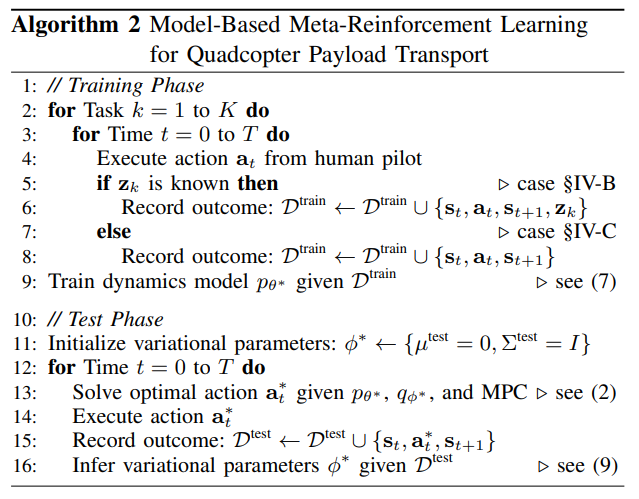
Method Implementation
Payload Variations
- 3D printed payloads weighing between 10-15 grams.
- Experiments vary primarily the string length between 18-30cm long (18cm or 30cm). (since the dynamics are more sensitive to string length than mass)
Data Collection Spec.
- actions \(a \in \mathbb R^3\) : Cartesian velocity commands
- states \(s \in \mathbb R^3\) : pixel location \(\mathbb R^2\) X size of the payload \(\mathbb R\)
Dynamic Model \(p_\theta\) and MPC Details
- NN consists of four FC hidden layers of size 200 with swish activations (also known as SeLU).
- MPC is run with a time horizon of 5 steps, using the cross entropy method to optimize, with a sample size 50, selecting 10 elite samples and 3 iterations.
- MPC computation takes 50-100ms -> select control frequency to be 4Hz for both training and test time -> 150-200ms for latent variable inference
Experimental Evaluation
Aims of Experiments
- Q1 Does online adaptation via meta-learning lead to better performance compared to non-adaptive methods?
- Q2 How does our meta-learning approach compare to MBRL conditioned on a history of states and actions?
- Q3 How does our approach with known versus unknown dynamics variables compare?
- Q4 Can we generalize to payloads that were not seen at training time?
- Q5 Is the test-time inference procedure able to differentiate between different a priori unknown payloads?
- Q6 Can our approach enable a quadcopter to fulfill a complete payload pick-up, transport, and drop-off task, as well as other realistic payload transportation scenarios?
Baseline Approaches
- MBRL: state consists of only the current payload pixel location and size
- MBRL with history: simple meta-learning approach, where the state consists of the past 8 states and actions concatenated together
- PID controller: three PID controllers for each Cartesian velocity command axis. PID gains are manually tuned by evaluating the performance of the controller on a trajectory following path not used in this experiments for a single payload.
Trajectory Following
- Tracking specified payload trajectories: a circle or square path in the image plane or a figure 8 path parallel to the ground (with a suspended cable either 18cm or 30cm long)
- Used a latent variable of dimension one
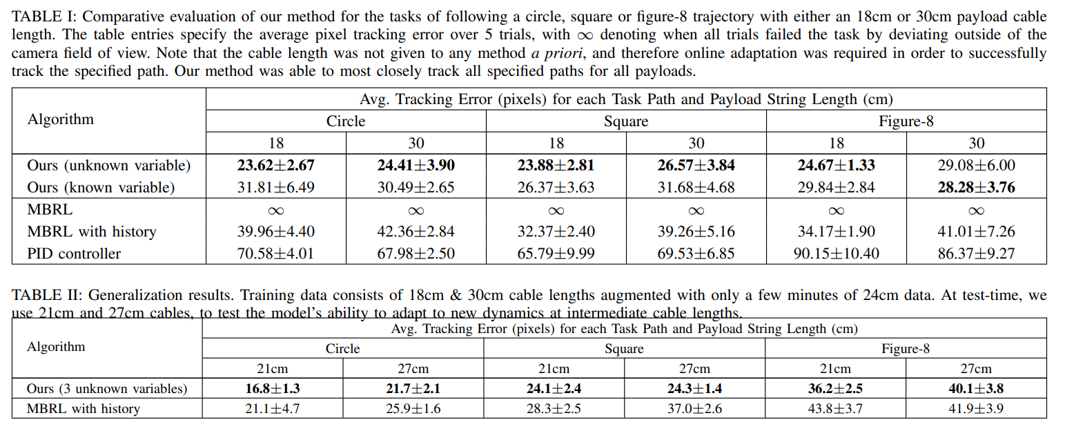
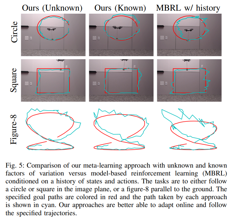
- Both the online adaptation methods(=the proposed method and MBRL with history) better track the specified goal trajectories compared to the non-adaptation methods(=MBRL and PID controller)(Q1).
- The proposed method outperforms the other meta-learning method MBRL with history (Q2).
- The proposed method with unknown latent variables at training time outperforms the proposed method with known latent variables (Q3). Inferring unknown latent variables at training-time might captures unspecified types of variation from potentially hard to observe factors.
- The proposed method has an ability to generalize to new payloads not seen during training (Q4). Learning how string lengths affect the dynamcis benefited from a few minutes of data from a third (24cm) string length, allowing the algorithm to rapidly interpolate to unseen string lengths of 21cm or 27cm at test-time, shown in Table 2.
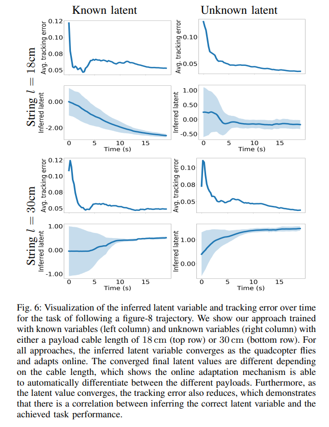
- The dynamic variable converges to different values depending on the cable length, which shows that the test-time inference procedure is able to differentiate between the dynamics of the two different payloads (Q5).
- As the inferred value converges, the learned model-based controller becomes more accurate and is therefore better able to track the desired path (Q1).
End-to-End Payload Transportation
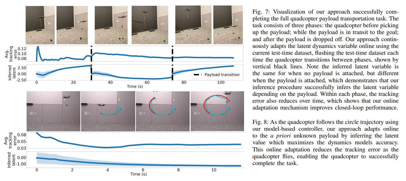
- The proposed method successfully completes the full task (Q6) due to the online adaptation mechanism (Q1, Q5).
- Each time the quadcopter transitions between transporting a payload and not transporing a payload, the quadcopter re-adapt online to be able to successfully follow the specified trajectories.
Additional Use Cases
- Additional payload transportation cases are available on
the authors' website - The proposed method is able to transport a suspended payload (Q6): towards a moving target, around an obstacle by following a predifined path, and along trajectories dictated using a “wand”-like interface.